Mining Software Repositories

3 posts with the tag “Mining Software Repositories”

Building an ownership cartography of a system - Part 2

Aug 13, 2026

When you share your work with others, such as the previous blog post, you can get feedback and suggestions for improvement. And this is exactly what happened.

And by Distribution Map, we are talking about a research paper accepted at ICSM 2006 So, let’s not reinvent the wheel anymore and look at how to use the already existing Distribution Map in Moose to visualize the ownership of a system.

One color for each developer

The first visualisation that comes to mind is to use one color for each developer. Using the Degree-of-Authorship (DOA) formula, we can compute the ownership of each file and retrieve the main developer for each file.

In moose, we can then create a tag that will associate a color to each developer and then use this tag to color the files in the system. We assign a tag to each file that corresponds to the main developer of the file.

((glhModel allWithSubTypesOf: GLHFile)
    select: [ :file | file diffs size ~= 0 ])
  do: [ :file |  file tagWithName: ((file degreeOfAuthorship) keyAtValue: 1.0) name  ].

We first search for all the files that have been modified, then we compute the degreeofAuthorship for every possible user, we select the one with the best score, which is 1, and we create a tag with the author name. Once the tag is created for every file, it is possible to propagate the files to the Distribution Map.

Propagate to Distribution Map

To propagate the files to the distribution, we first retrieve the files in our model. Then, we get the parent folder of the files.

appsFolder := (glhModel allWithSubTypesOf: GLHFileDirectory) detect: [ :fi | fi path = 'src' ].
files := (appsFolder allToScope: GLHFileBlob).
"Find parent folder"
folders := (files collect: [ :file | file directoryOwner ] as: Set).
folders

Based on the parent folders, the Moose Distribution Map will be able to recalculate the children, and so the files of interest. We select the folders variable and propagate with Cmd + Shift + M, Cmd + Shift + P.

Then, we open the Distribution map from the Moose Menu.

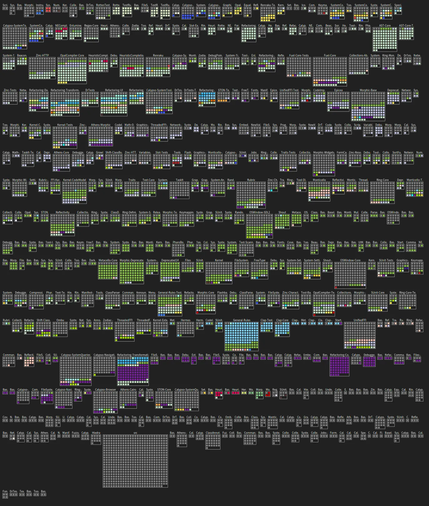
We first get a visualisation without any color. So, in the settings of the visualisation, we select the tags to display. We select every authors and get the last visualisation.

visu

Again, the visualisation well presents the different packages and the one with major author. The gray square corresponds to file less modified in the system the last two years.

Building an ownership cartography of a system

Aug 11, 2026

Benoit Verhaeghe

Moose expert

Context

When managing a software system, it is important to know who is responsible for which part of the system. This information can be useful for various reasons, such as identifying potential bottlenecks, understanding the impact of changes, and improving collaboration among team members.

One major threat could, for example, come from a developer leaving the team. This is often referred to as the “bus factor” or “truck factor”. But how to detect such a situation?

Research have shown that the ownership of a system can be inferred from its version control history. To do so, one approach is to first investigate the ownership of each file.

Two nice papers, not from the Moose community, are:

Computing the ownership of a file

Looking at the research paper, we can find a formula that can help build a first version of ownership. It consists for each file of a git repository to compute a degree of authorship for each potential author using this formula.

Given a file $f$ with path $f_p$ , the degree-of-authorship of a developer $d$ whose Git user has been mapped to $m_d$ is given by.

DOA(m_d, f_p) = 3.293 + 1.098 × FA(m_d, f_p) + 0.164× DL(m_d, f_p)−0.321 ×ln(1 + AC (m_d, f_p))

With the following definitions:

DOA depends on three factors: (i) first authorship ( $FA$ ): if $m_d$ originally created $f$ , $FA$ is 1; otherwise it is 0; (ii) number of deliveries ( $DL$ ): number of changes in $f$ made by $m_d$ ; and (iii) number of acceptances ( $AC$ ): number of changes in $f$ made by any developer, except $m_d$ .

Looking at the source code of the Truck-Factor tool, we can see thet $DL$ corresponds to a commit that modifies a file. The file can be added, modified, and renamed.

$AC (m_d, f_p)$ is computed by the total number of modifications of a file minus the number of modifications made by the developer $m_d$ .

Moose Implementation

Moose comes with the GitProject Health project to represent a Git repository and analyze its history. So, I wanted to implement the DOA formula in Moose.

Making it faster

One concern is that GitProject Health is firstly made to analyze Git Social Platform and not only git repository with the truck factor in mind. Thus, it is not optimized for this use case.

The major concern comes when loading the model that rely on several calls to the Git Platform API. In order to avoid this, I decided to implement a companion importer named GitLocalModelImporter that can load a model from a local git repository.

To go faster, it relies on the FFI LibGit2. This project includes a LGitRevwalk, a walker that can iterate over the commits of a git repository. Thus, we can iterate over the commits and retrieve the files, the diffs, the commits, and the authors in a repository.

This version is still not optimized to compute truck factor, but it can be used to do lot more than just computing truck factor. It comes as a new classic importer for GitProject Health and so can be used side by side with other importers for optimization.

Implementing the DOA formula

To implement the DOA formula, I created a simple but effective class named GLPDegreeOfAuthorshipAnalyzer. This class is now part of the GitProject Health project set of metrics. It reuses the exact same algorithm as the Truck-Factor tool to compute the degree of authorship for each file in a git repository.

We note several additionnal considerations to compute the DOA formula. These considerations are mention because they enable analysis of a project without considering the history of the project, which is long to consider.

The first authorship ( $FA$ ) is computed by looking at the first commit that added or modified a file to the repository.
GitProject Health does not consider renaming of files yet, so it does not consider file renaming.

Even though not considering rename can create issues, this work has been performed on an industrial project and considering renaming would not drastically change the results of the analysis.

Vizualizing the ownership of a system

The last step I wanted to investigate is to visualize the ownership of a system. I did not create a vizualization dedicated to this point yet. But let’s investigate a running example for the pharo project.

After cloning the project, I create a Moose image with the GitProject Health project installed. Then, I load the pharo project.

glhModel := GLHModel new.
repository := GLHRepository new
    cacheAt: #localImporterReference
    put: '/path/to/MSR/pharo' asFileReference;
    yourself.

glhModel add: repository.

localImporter := GitLocalModelImporter new.
localImporter withFiles: true.
localImporter glhModel: glhModel.
"I will import the last two years"
localImporter withCommitsSince: 2 years.
localImporter importRepository: repository.

After a possibly long execution, we get the repository loaded. It is thus possible to investigate it using our tools.

We want to build a cartography of the application to identify the coverage of files with an author. To do so, I decided to build a TreeMap using the Roassal framework.

First, I need to load the Roassal TreeMap support

Metacello new
    baseline: 'Roassal';
    repository: 'github://pharo-graphics/Roassal:Pharo13';
    onConflictUseIncoming;
    load: #( Full )

Then, start the fun.

A quick view of the project

We build a dictionary with the degree of authorship for everyfile.

filesAuthorShip := ((glhModel allWithSubTypesOf: GLHFile)
    select: [ :file | file diffs size ~= 0 ])
    collect: [ :file |
        "This uses our analyser behind the scene"
        file -> file degreeOfAuthorshipAuthors ]
    as: Dictionary.

We look for the folder that is the root of the tree map, and we compute the max number of authorship that will be used for coloring the vizualisation.

appsFolder := (glhModel allWithSubTypesOf: GLHFileDirectory)
    detect: [ :fi | fi path = 'src' ].

max := (filesAuthorShip collect: #sum) max.

Finally, we build the tree map.

palette := RSQualitativeColorPalette qualitative set39.
b := RSTreeMap new.
b inset: 2 asPoint.
b boxShape borderColor: Color black.
b boxShape borderWidth: 0.05.

color := NSScale linear domain: { 0. max };
    range: #( white red ).
b
    leafWeight: [ :f | 1 ];
    explore: appsFolder nesting: [ :directory |
        directory files select: [ :f | (f isKindOf: GLHFileDirectory) ] ]
    leaves: [ :directory | directory files reject: [ :f | f isKindOf: GLHFileDirectory ] ].

b shapes
    do: [ :box |
        box borderWidth: 1.
        box isSLeaf
            ifTrue: [ box color: (color scale: (filesAuthorShip at: box model ifPresent: [ :dic | dic sum ] ifAbsent: [ 0 ])) ]
            ifFalse: [
                | path |
                path := (box model path splitOn: '/').
                path size > 1 ifTrue: [
                    box color: (palette scale: (box model path splitOn: '/') second) ] ] ].

b shapes @ (RSPopup text: [:f | f path, String crlf, ((filesAuthorShip at: f ifPresent: [ :dic | dic sum ] ifAbsent: [ 0 ]) printString) ]).

b build

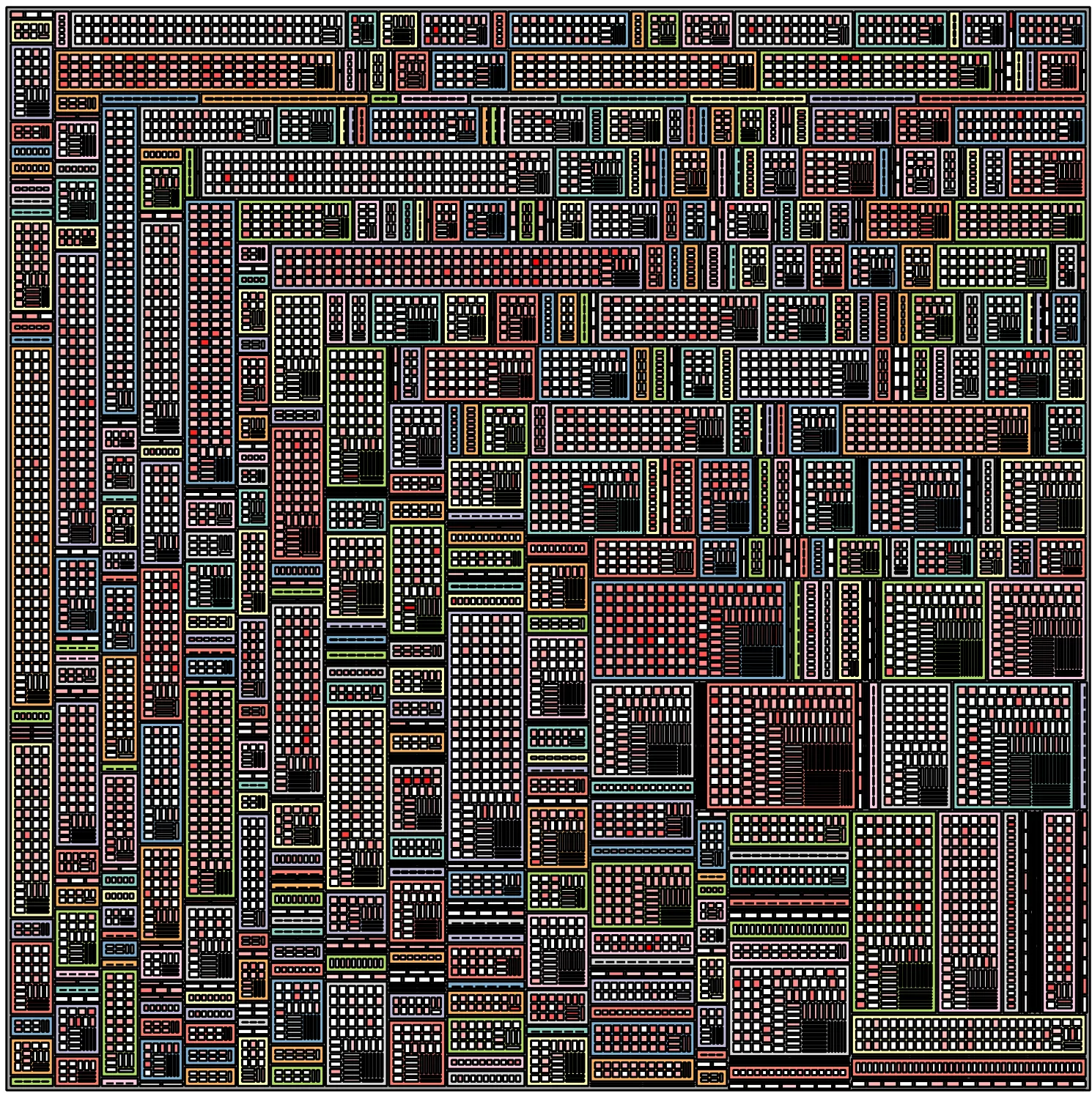
Using this script, we built a vizualisation with different color for each package, and a red scale for know packages. It ouput the following image

"Result"

Looking at the image we see that some package have author from the 2 last year modification whereas other were not modified at all.

More than showing the Truck Factor, this vizualization highlights the code that have been updated by people that gain or conserve knowledge on the codebase.

One improvment could be to highlight the core contributors.

highlighting the core contributors

To highlight the core contributors, we first create a color palette for them.

coreContributors := (filesAuthorShip values flatCollect: #keys) asSet.
paletteContributor := RSQualitativeColorPalette qualitative flatui120.

Then, we update the first b shapes statements by:

b shapes
    do: [ :box |
        box borderWidth: 1.
        box isSLeaf
        ifTrue: [
            filesAuthorShip at: box model ifPresent: [ :dic |
                | author |
                author := (dic associations sorted: [ :a :b | a value > b value ]) first key.
                box color: (paletteContributor scale: author) ] ]
        ifFalse: [
            | path |
            path := (box model path splitOn: '/').
            box color: Color white ] ] ].

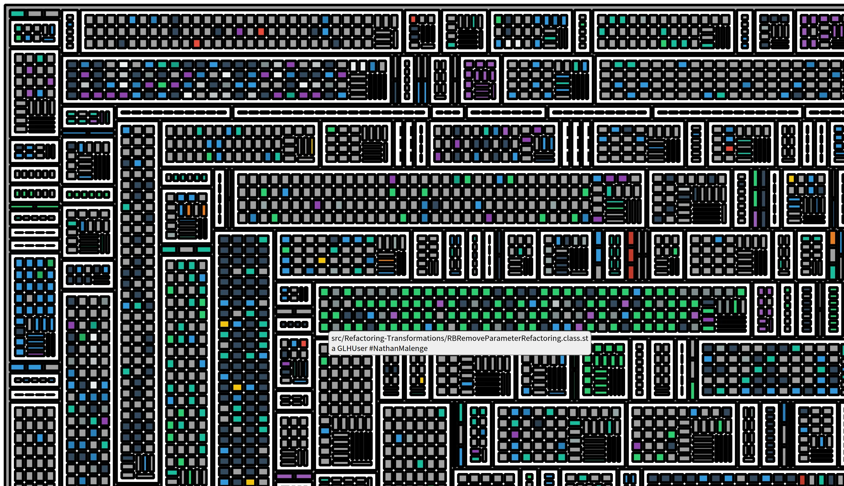
This attributes the color of the core contributors to each box. We present below a final computed visualization that highlight one contributor who seems to became the expert of the Refactoring package.

Core Contributor

First look at GitProjectHealth

Mar 24, 2025

Benoit Verhaeghe

Moose expert

When it comes to understand a software system, we are often focusing on the software artifact itself. What are the classes? How they are connected with each other?

In addition to this analysis of the system, it can be interesting to explore how the system evolves through time. To do so, we can exploit its git history. In Moose, we developed the project GitProjectHealth that enables the analysis of git history for projects hosted by GitHub, GitLab, or BitBucket. The project also comes with a set of metrics one could use directly.

First use of GitProjectHealth

GitProjectHealth is available in the last version of Moose, it can be easily installed using a Metacello script in a playground.

Metacello new
  repository: 'github://moosetechnology/GitProjectHealth:main/src';
  baseline: 'GitLabHealth';
  onConflict: [ :ex | ex useIncoming ];
  onUpgrade: [ :ex | ex useIncoming ];
  onDowngrade: [ :ex | ex useLoaded ];
  load

Example on Famix

For this first blog post, we will experiment GitProjectHealth on the Famix project. Since this project is a GitHub project, we first create a GitHub token that will give GitProjectHealth the necessary authorization.

Then, we import the moosetechnology group (that hosts the Famix project).

glhModel := GLHModel new.

githubImporter := GithubModelImporter new
  glhModel: glhModel;
  privateToken: '<private token>';
  yourself.

githubImporter withCommitsSince: (Date today - 100 days).
group := githubImporter importGroup: 'moosetechnology'.

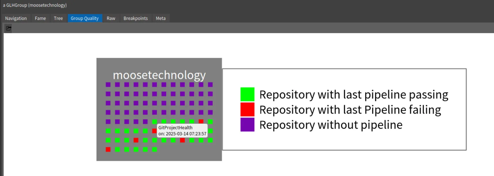
This first step allows us to get first information on projects. For instance, by inspecting the group, we can select the “Group quality” view and see the group projects and the last status of their pipelines.

Group Quality view for moosetechnology

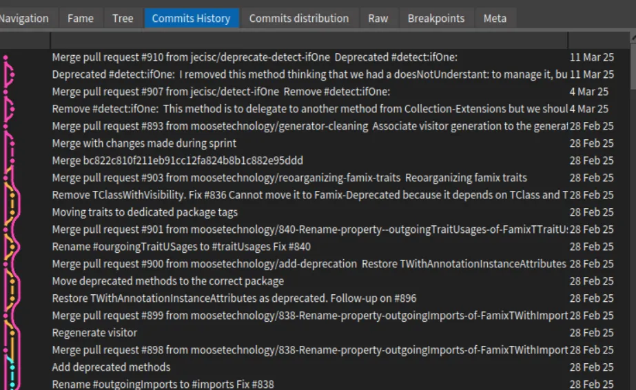
Then, by navigating to the Famix project and its repository, you can view the Commits History.

alt text .

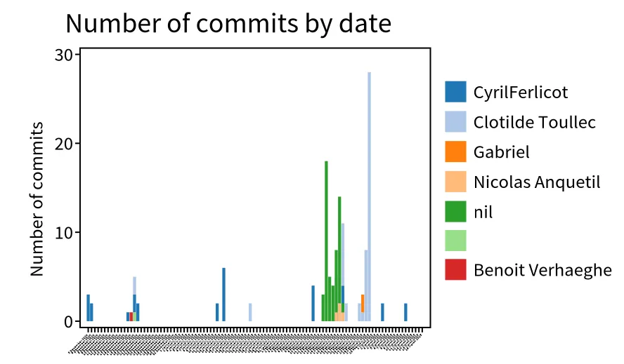
It is also possible to explore the recent commit distribution by date and author

commit distribution .

In this visualization, we discover that the most recent contributors are “Clotilde Toullec” and “CyrilFerlicot”. The “nil” refers to a commit authors that did not fill GitHub with their email. It is anquetil (probably the same person as “Nicolas Anquetil”). The square without name is probably someone that did not fill correctly the local git config for username.

Who modified my code? - code churn

A popular metric when looking at git history is the code churn. Code churn refer to edit of code introduced in the past. It corresponds to the percentage of code introduced in a commit and then modified in other comments during a time period (e.g in the next week). However many code churn definitions exit.

The first step is thus to discover what commits modified my code. To do so, we implemented in GitProjectHealth information about diff in commit.

To extract this information, we first ask GitProjectHealth to extract more information for the commits of the famix project.

famix := group projects detect: [ :project | project name = 'Famix' ].

"I want to go deeper in analysis for famix repository, so I complete commit import of this project"
githubImporter withCommitDiffs: true.
famix repository commits do: [ :commit | githubImporter completeImportedCommit: commit ].

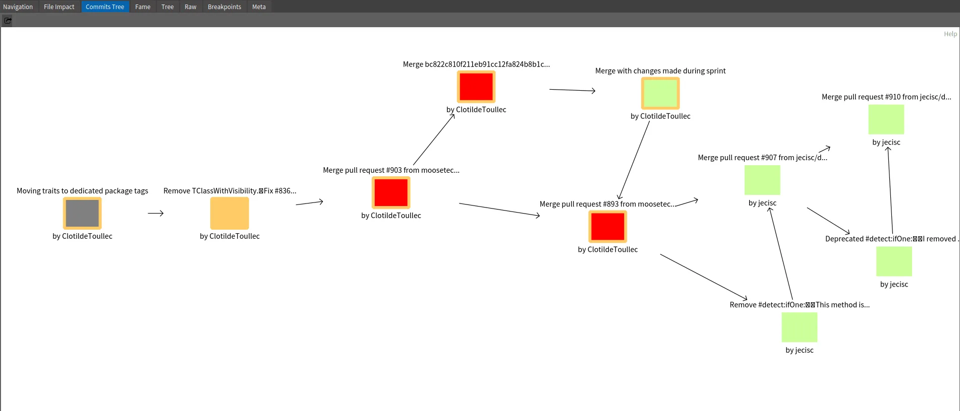
Then, when inspecting a commit, it is possible to switch to the “Commits tree” view.

Commit Tree

Here how to read to above example

The orange square “Remove TClassWithVisibility…” is the inspected commit.
The gray square is the parent commit of the selected ones.
The red squares are subsequent commits that modify at least one file in common with the inspected commit
The green squares are commits that modifies other part of the code

Based on this example, we see that Clotilde Toullec modifies code introduced in selected commits in three next commits. Two are Merged Pull Request. This can represent linked work or at least actions on the same module of the application.

Can we go deeper in the analysis?

Connect GitProjectHealth

It is possible to go even deeper in the analysis by connecting GitProjectHealth with other analysis. This is possible by connecting metamodels. For instance, it is possible to link GitProjectHealth with Jira system, of Famix models. You can look at the first general documentation, or stay tune for the next blog post about GitProjectHealth!