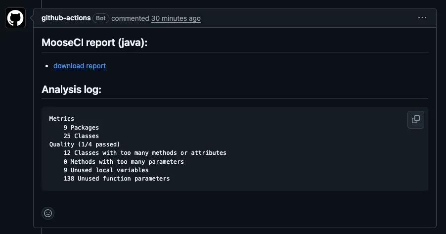
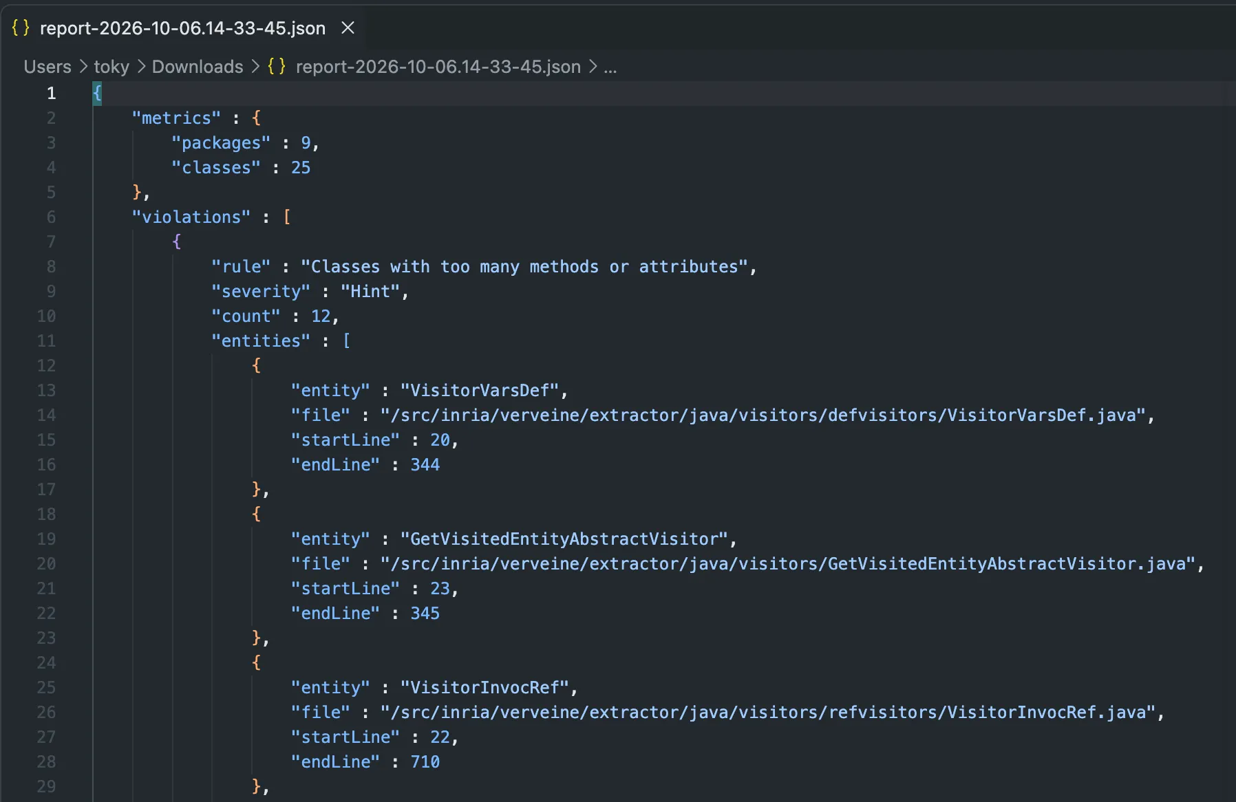
MooseCI is easy to use. You can run it locally with Docker, or on every pull request with the GitHub Action. You only need a configuration file and a small workflow.
Static Single Assignment is a program representation where every variable is assigned exactly once. The same logical variable x is renamed into several versionsx_1, x_2, … — one per assignment — and each use points to the version that can actually provide its value.
The goal is to make data flow explicit in the AST: instead of “this x is assigned somewhere before”, we get “this x is exactly the value produced by that assignment”.
x =2# x_1
print(x) # uses x_1
x =3# x_2
print(x) # uses x_2
The hard part starts when the value of a variable can come from several assignments depending on the control flow:
if z >3:
x =2# x_1
else:
x =3# x_2
print(x) # uses phi(x_1, x_2)
After the merge of the two branches there is no single assignment that produced x: we say x has a phi versionphi(x_1, x_2), a virtual assignment stating “the value is x_1 if we came from the first branch, x_2 if we came from the second”. An analysis consuming the SSA can then explore both possible values.
For us, the SSA is the third stage of the pipeline, sitting on top of the two previous stages:
Import → Local resolution → CFG → SSA
It has a hard prerequisite: we must know, for each use, which declaration it refers to (the local resolution stage) and which control-flow paths exist (the CFG stage). If you have not read about the FAST CFG and its visitor, I strongly recommend the Visiting the control-flow graph article first — this blog post is the direct continuation.
The whole transform lives in a single class, FASTPythonSSAVisitor. Its declaration shows the trick that makes it work: it combines two visiting abilities—
FASTPythonVisitor <<#FASTPythonSSAVisitor
traits: 'FASTCFGTVisitor';
slots: { #newVariablesMap. #localDeclarations };
tag: 'CFG/LocalResolver/SSA';
package: 'FAST-Python-Tools'
the superclass FASTPythonVisitor brings the language visitor (the visitFASTPyXxx: methods generated from the model, through FASTPyTVisitor);
the trait FASTCFGTVisitor brings the CFG visitor (the visitCFGXxxBlock: methods that walk the blocks of the CFG, plus the conditional-branch hooks).
So a single accept: can traverse the CFG (visitCFGBlock: and friends) and, when a block contains Python statements, dispatch back to the language-specific visit methods (visitFASTPyAssignment:, visitFASTTCanBeVariable:, …).
The trait is generic and lives in the base FAST project (FAST-Core-Tools), which means any language model can reuse it the same way. It is the same trait-based composition idea as the local resolver, but applied to the CFG.
localDeclarations — an IdentitySet of every local declaration that received at least one SSA version while walking the entity. It is the source of the “current active versions” snapshot (see below).
newVariablesMap — an IdentityDictionary used only during the merge of conditional branches, to accumulate, per branch, the versions that were created inside that branch.
The versions are not strings, they are first-class objects living in FAST-Core-Tools (again reusable across languages), and they are Moose entities: each version is added to the model, so it is persisted and exported with it.
FASTAbstractVariableVersionSSA — abstract root. It holds the localDeclaration the version belongs to, and offers the queries we need once the SSA is built: nodes (the accesses directly linked to this version, the bidirectional opposite of ssaVersion), localUses, readAccesses, writeAccesses (restricted to this version), name, isPhi, ssaVariables.
FASTVariableVersionSSA — a basic version for one assignment. It carries an integer version number, so name answers x_1, x.y_1…
FASTVariablePhiVersionSSA — a phi version. It carries choices, the collection of versions being merged, so name answers phi(x_1, x_2), and isPhi answers true.
FASTVariableVersionSSA >> name
^ String streamContents: [ :s|
s
nextPutAll: self localDeclarationName;
nextPut: $_;
nextPutAll: version asString ]
FASTVariablePhiVersionSSA >> name
^'phi(', ($, join: (choices collect: #name)) ,')'
Nested merges flatten themselves: the phi’s addChoiceToPhi: re-dispatches each choice into the receiving phi, so a phi inside a branch ultimately contributes its own choices to the outer phi.
The SSA result is attached to the model through two links defined in FAST-Core-Tools on the trait FASTTCanBeLocalDeclaration (used by FASTTEntity, so available on every FAST entity):
entity ssaVersion — on any access (read or write) to a variable, the version it is linked to. This is a bidirectional relation: each version exposes the accesses linked to it through its nodes collection.
declaration activeVersion — on the local declaration, the current version at the current point of the traversal. This is the internal “state variable” of the algorithm: it is bumped at each assignment and replaced by a phi at each merge. It stays a plain attribute.
The SSA is then a traversal that, at every write, creates a version, adds it to the model, and sets it as activeVersion; at every read, copies activeVersion into ssaVersion of the access.
Just like the local resolver, the SSA logic is concentrated on the trait FASTTCanBeVariable, caught in a single visit method for every node kind that can be a variable (identifier, attribute access, subscript, walrus):
The rule is a direct SSA translation of the local resolver’s “write declares, read binds”:
write access → create a new version (handleNewAssignemntTo:);
read access → copy the declaration’s activeVersion into the access’s ssaVersion;
read of an unresolved name (localDeclaration isNonLocalDeclaration) → nothing. print, len, imported functions and variables have no declaration in the model, so they get no version (ssaVersion stays nil);
first read of a subscript whose declaration has no version yet → it behaves like a declaration: the first x[3] read is treated as an assignment (mirroring the local-resolver convention), so its version is created there.
FASTVariableVersionSSA for: aFASTEntity records aFASTEntity localDeclaration as the declaration the version belongs to. Then:
the new version is added to the model — the versions are Moose entities, so this makes them persistent and exported with the model;
the version number is seeded from lastSSAVersion — the active version of the previous declaration of the same name, chased through the local-resolver shadowing chain: it is what makes x_1 then x_2 even when an unrelated def x(): was declared in between;
the new version becomes the activeVersion of the declaration;
the declaration is added to localDeclarations (so the “snapshot” of active versions, used for the branches, sees it);
newVersionNumber bumps the integer — version := version + 1 — and the result is stored as the write access’s ssaVersion.
FASTPyEntity >> lastSSAVersion
"scrolling the shadowing chain of the declaration to find a previous version"
| entity |
entity :=self localDeclaration.
[ entity isNotNil ] whileTrue: [
entity activeVersion ifNotNil: [ :version|^ version ].
The generated visitor visits the children of a node in metamodel order. For the SSA, that order is often wrong because a read must be resolved against the versions before the node, and a write must only bump the version after its right-hand side has been read. We overwrite the generated visit methods in four places.
This is the most important one. In the metamodel, the left of an assignment comes before its right. For the SSA we must invert:
visitFASTPyAssignment: anAssignment    "Visiting the right field before the left because the variables at the     right should be linked to the previous assignment."    self visitFASTPyTAssignable: anAssignment.    self visitFASTPyExpression: anAssignment.
    self visitEntity: anAssignment right.    self visitEntity: anAssignment left.    self visitEntity: anAssignment type
Consider x = x + 1. In metamodel order we would visit the left x first: it would create x_2 and set it as activeVersion, and then the x in x + 1 would read — wrongly — the new x_2. By visiting right before left, the read sees x_1 and the write bumps afterwards.
A function definition appearing as a statement of the module is inside the module CFG. But the function’s body is a separate control-flow world. When we reach a definition, we therefore rebuild a fresh CFG and restart the traversal on it, so each definition is turned into its own SSA form:
Where do phi versions come from? The CFG visitor. When FASTCFGTVisitor visits a conditional block, it visits all the branches before the merge, and during that it calls four hooks you can override. Their default implementation in the trait is empty:
preConditionalsBranchesVisitOf: aConditionalBlock "before the first branch"
preConditionalsBranchVisitOf: block conditional: aConditionalBlock "before each branch"
postConditionalsBranchVisitOf: block conditional: aConditionalBlock "after each branch"
postConditionalsBranchesVisitOf: aConditionalBlock "after all branches, before the merge"
That is exactly the machinery we fill in to build phis. The idea is a three-step protocol:
before the branches: snapshot the active versions;
after each branch: record which new versions were created by that branch;
after all branches: merge, per variable, one version per branch (plus the snapshot version for branches that did not assign it) into a phi.
The difference is atomic: subtracting the snapshot (#previousVariables) from the current active versions leaves exactly the versions created inside this branch (the ones that were not there before). We store them per branch block.
declarationsToMerge — the set of distinct local declarations that received at least one new version in some branch;
for each such declaration, walk the branch map and gather the one version per branch that belongs to it;
if not every branch created a version for it, a branch may fall straight through with the old value — so we also merge in the version that was active before the conditional (from the previousVariables snapshot), if it existed;
if a single candidate version remains (e.g. only one branch assigns, and merging the previous version produces a single version) there is nothing to merge, so no phi is created — the single version just stays active;
otherwise a FASTVariablePhiVersionSSA is created with the candidate versions as choices, and becomes the new activeVersion of the declaration — so the reads right after the merge pick it up via the normal “copy activeVersion into ssaVersion” rule.
No need to “attach” anything else: the phi inherits from the version classes, so it knows its localDeclaration and exposes localUses, readAccesses, writeAccesses restricted to the merged versions.
preConditionalsBranchesVisitOf: → previousVariables snapshot is empty (no version yet).
then branch: x = 4 → handleNewAssignemntTo: creates x_1, becomes active.
postConditionalsBranchVisitOf: → branch recorded with {x_1}.
else branch: x = 5 → creates x_2, becomes active.
postConditionalsBranchVisitOf: → branch recorded with {x_2}.
postConditionalsBranchesVisitOf: → declaration merged: {x_1} from branch 1, {x_2} from branch 2 → both branches assigned, so no previous version added → allVersions = {x_1, x_2} → phi created, becomes active.
print(x) is read after the merge → ssaVersion := activeVersion → phi(x_1, x_2). The use is linked to both possible values.
And the case where a branch does not assign the variable:
x =3# x_1
if y <2:
function() # no assignment of x
else:
x =4# x_2
print(x) # phi(x_1, x_2)
Step 6 here: branch 2 introduced x_2 only, and branch 1 introduced none for x → allVersions starts as {x_2}, its size (1) is not the number of branches (2) → we add the previous version x_1 from the snapshot → allVersions = {x_1, x_2} → phi. Correct: if the first branch is taken, x still holds the old value.
If the assignment happens in a single branch and no previous version exists, then allVersions ends up with a single element → no phi, and the reads just use that single version — matching the (correct) semantics that the variable is simply that assignment in all reachable paths.
Once the SSA is built, the model can be queried directly:
access ssaVersion — the version of the access: a FASTVariableVersionSSA or a FASTVariablePhiVersionSSA (or nil for unresolved names and non-local declarations).
access ssaName — its pretty name, e.g. x_1, x.y_2, phi(x_1, x_2).
version nodes — the accesses directly linked to this version through ssaVersion (the bidirectional opposite).
version localUses / version readAccesses / version writeAccesses — the accesses for this specific version (in the phi case, over all its choices).
model allSSAVersions / model allResolvedVariableVersions — all the versions of the model, the latter without duplicates.
variable allSSAVersions / variable allSSABasicVersions — all versions of one variable, the latter without the phis.
The SSA inherits the limitations of the two stages it sits on:
Instance variables (self.x) cannot be treated correctly: there is no declaration of them, and we do not know the order in which methods are invoked.
Subscripts are matched by their source code, so x[a] and x[b] are conflated — and the whole “first read acts as a declaration” convention is a workaround, not a real answer.
Non-local declarations get no version: unresolved and imported names are invisible to the SSA.
Attribute access chains are not tracked (a = x.y then a.z is not linked to x.y.z).
Reuse the generic machinery.FASTCFGTVisitor, FASTVariableVersionSSA, FASTVariablePhiVersionSSA and the version queries live in the base FAST project (FAST-Core-Tools). You should only have to write the language-specific part: the visitX: rules for your nodes and the branch hooks.
The write/read rule is your whole core. One visit on the trait “can be a variable” (read → copy active version, write → create version) is enough, provided the local resolution already linked uses to declarations.
Drive phis from the CFG hooks, not by scanning. The four pre/postConditionals* hooks give you the branch boundaries for free. Snapshot before, record per branch, merge after — that protocol is generic.
Order your visits so reads see the old version. The metamodel order is a trap: reorder assignments (right before left), functions (parameters before body), and anything that mixes declaration and use.
Give each access a version and each declaration a “current version” attribute. A ssaVersion relation (bidirectional with nodes) and an activeVersion attribute on FASTTCanBeLocalDeclaration were enough. Make the versions Moose entities and add them to the model so they are persisted and exported.
Make the versions first-class objects, not strings. Give them a localDeclaration, name, and ssaVariables/choices; the query API (localUses, readAccesses, …) then comes almost for free on the abstract root.
Handle your “no declaration” case explicitly. In Python, unresolved/imported names simply get no version. Decide early what your language’s equivalent is (a non-local placeholder, an explicit global scope…).
The FAST-Python sources you will want to look at: FASTPythonSSAVisitor (this post is a guided read of it), the FASTCFGTVisitor trait and the FAST*VersionSSA classes in FAST-Core-Tools, and the SSA tests in FASTPythonSSATest.
This implementation currently lives in FAST-Python, but almost everything in it could move to the base FAST project in the future.
The language-specific part is surprisingly thin. Given a CFG, a local resolution, and a model whose variables use the FASTTCanBeVariable trait, this SSA implementation gives you almost everything for free:
the version classes (FASTVariableVersionSSA, FASTVariablePhiVersionSSA) and the FASTCFGTVisitor trait already live in FAST-Core-Tools;
the write/read rule is a single visit method on FASTTCanBeVariable;
the phi building runs on the generic CFG hooks.
So, for a new language, there is almost nothing more to do: mostly override the few visitX: methods where the metamodel order is wrong for SSA — assignments (right before left), functions (parameters before body), and definitions (rebuild their own CFG) — to reorder the visits.
The goal of this blog post is to explain how I implemented a local resolver for FAST-Python. FAST-Python is on of the hardest project to implement this kind of algo, so reading this should help implementing any other local resolver for other languages.
Local resolution is a symbol resolution pass: it links each named entity to the entity that declares it. In other words, for every occurrence of a name — read, write, call, import — it answers the question “where does this name come from?”.
In FAST-Python, after the model is imported from source, running the local resolver produces a model where every name usage points to its local declaration:
x =1# this is the declaration of `x`
print(x) # this use of `x` is linked to the declaration above
It is called local because it only resolves declarations that live in the same file/model (in contrast to a global/system resolution that would also resolve calls to external libraries, standard modules, etc.). Once we went through the file, a name that is not declared anywhere in the file gets bound to a special FASTNonLocalDeclaration placeholder — it is a declaration for the model, but we know it refers to something outside.
Local resolution is the foundation on top of which our other analyses are built such as the Static Single Assignment (SSA). Without it, you cannot even tell whether two x in the code are the same variable. You can’t even say if a FASTPyIdentifier is a variable or not.
The result of the resolution is exposed through two accessors available on every FAST entity (they live in the FAST-Core-Tools package of the base FAST project, so they are reusable across languages):
entity localDeclaration — from any use of a name, returns the entity that declares it (the first assignment, a FASTPyFunctionDefinition, a loop variable, an import…). If the name was not declared in the file, it returns a FASTNonLocalDeclaration.
declaration localUses — from a declaration, returns all the entities that resolve to it (usages and other declarations that share it).
This is a bidirectional relationship: localUses is the exact inverse information of localDeclaration.
On top of those two, FAST-Python adds a set of convenience queries that only make sense once the resolution is done — and only for nodes that represent variables:
access allAccesses / allReadAccesses / allWriteAccesses — all the read/write accesses to the same variable.
access internalAccesses — the attribute accesses and subscripts on the variable (x.y, x[3]).
access allNodesUsingMe / access allStatementsUsingMe — the statements that use the variable.
variable isResolvedVariable — true if the node resolves to a local variable declaration (and is not a function, method, import or unresolved name).
node usedVariables — all the entities in the subtree of the node that resolve to local variables.
The resolver is implemented as a Moose/FAST visitor: FASTPythonLocalResolverVisitor. It visits a FAST model (a FASTPythonVisitor built on the generated visitor trait FASTPyTVisitor) and inspects/annotates the nodes in place.
If you are not familiar with how the visitor is generated from the model, I strongly recommend reading Improving the Visitor Generator first: it explains how FASTPyTVisitor is produced and how you can override the generated visitX: methods.
The Python problem: there is no declaration of variables
Before we can write a single line of the algorithm, we have to deal with the first (and deepest) Python quirk: there is no declaration of variables.
In Java you get a real declaration:
intx=1; // I declare and type `x`
In Python, an assignment is the declaration:
x =1# this IS the declaration of `x`
There is no keyword, no type, no way to distinguish “declare a fresh variable” from “reassign an existing one” syntactically — the same syntax x = ... does both. The resolver has to decide, and the decision is purely lexical reasoning about scopes and order, with no syntactic marker to lean on. Concretely:
The first assignment in a scope is the declaration. The resolver must therefore know the order in which things appear, and which construct “creates” a scope.
Parameters are declarations: def f(x): ... declares x as the function’s parameter. They are semantically the first assignment in the function’s scope.
Walrus operators (x := ...) declare x inline, even inside an expression or an if condition.
A for ... in ... loop declares its target variable — but only the first time; it must be a declaration when the variable is not already known in the scope.
Augmented assignments (x += 1) are uses + writes to the same variable.
For clauses in a list comprehension.
In our implementation this all boils down to a single rule expressed in visitFASTTCanBeVariable: (see below): a write access declares and bind, a read access binds. Everything else is scope management around that rule.
The superclass is FASTPythonVisitor (from the generated FASTPyTVisitor trait), so all the visitX: methods come for free: we only override the ones where the metamodel visit order differs from the resolution order.
namesContext is a stack of scopes (a Stack of Dictionarys, mapping name -> declaration). It is initialized in initialize:
When a read has no matching declaration in any scope, bind:...ifAbsentUse: falls back to ensureNonlocalDeclarationNamed::
ensureNonlocalDeclarationNamed: aName
^self
ensureDeclarationOf: aName
declaration: (FASTNonLocalDeclaration new
name: aName;
yourself)
in: namesContext first
Note the scope: namesContext first is the bottom of the stack, so a FASTNonLocalDeclaration behaves as if it were declared at module level — reads of an undeclared name in a function and at module level end up in the same place. Also note that the fallback for attribute accesses and subscripts is slightly different (see the heart): declarationForUndeclaredNode:named: creates a local declaration on the first read of a subscript when the receiving variable has a declaration, and only resorts to the non-local declaration otherwise:
declarationForUndeclaredNode: aNode named: aName
"In case of a subscript, if the receiving variable exists, we consider
that the first read access to the subscript is the declaration."
aNode isSubscript ifTrue: [
aNode value
localDeclarationifPresent: [ :decl|
^self ensureDeclarationOf: aName
declaration: aNode
in: namesContext top ]
ifAbsent: [ "Nothing, just let the non local declaration." ] ].
Everything that can be a variable in FAST-Python implements the trait FASTTCanBeVariable (identifiers, attribute accesses, subscripts, walrus…). The visitor intercepts them in one place, and this is where “write declares / read binds” lives:
self declarationForUndeclaredNode: node named: name ] ].
super visitFASTTCanBeVariable: aTCanBeVariable
Two details make Python specific here:
localDeclarationName is the name that will be used for scope lookup. It is not always the identifier text: an attribute access and a subscript use their source code as their name, so x.y and x[3] are treated as first-class “variables” (with known limits, see Limitations). Every named entity gets a default from the base FAST project (FASTTNamedEntity>>localDeclarationName returns #name); the Python classes only override it where the name is not the identifier:
"from FAST, the default for any named entity:"
FASTTNamedEntity >> localDeclarationName [ ^self name ]
isVariableWriteAccess decides whether a node is a write access or a read access. It comes from FAST (FASTTEntity>>isVariableWriteAccess), but it delegates to variableDeclaration which is an explicitRequirement — every FAST project must implement it for the node kinds that can be variable write accesses. In FAST-Python, each relevant class provides its own logic to walk up the AST and check whether it sits in a write position:
"FAST core — the API:"
FASTTEntity >> isVariableWriteAccess [
^self variableDeclaration isNotNil
]
FASTTEntity >> variableDeclaration [
"If I am a node representing a write access, I return the node
assigning me. Else I return nil."
^self explicitRequirement
]
"FAST-Python — an identifier checks whether it is the left side of
"The default on FASTPyEntity returns nil (not a write access):"
FASTPyEntity >> variableDeclaration [ ^nil ]
The interesting bit: for identifiers, variableDeclaration does not just check the immediate parent — it first walks through tuple/destructuring parents via selfOrTopmostAssignableCollection, so that in (a, b) = (1, 2) the individual a and b correctly return the tuple assignment as their declaration.
Reordering the visit, or dealing with Python scoping
Because the visitor is generated (see the visitor generator blog post), it visits the children of a node in the metamodel order. For a resolver, metamodel order is not always resolution order: a construct may declare a name in a part of the syntax that the generated visitor reaches too late (or too early) relative to its uses.
Our main tool is therefore: override the generated visitX: with a manual ordering of a few visitEntity:/visitCollection: calls — and be very careful about when to open a scope, because Python does not create a scope where you would expect one.
Python does not create a scope for blocks. An if, a while, a for body do not introduce a new scope:
if cond:
y =3
print(y) # 3, perfectly valid Python
Combine that with “assignment is the declaration” and you get leaks: a variable assigned inside an if branch or a loop is visible after the block. For the resolver this means no useNewScopeDuring: around branches — a name assigned in the then must be visible in the else and after the whole statement. What we do control is the order, which is important for shadowing: in an if, the semantics are
the condition (can use outer variables, and walrus operators can even declare variables!),
The for ... in ... statement declares its loop variable in the enclosing scope (there is no loop scope). i survives after the loop. So a for is simultaneously a scoping and a declaring construct: the resolver must declare the target (left) in the current scope — no push — and, since that is the declaration, visit it before the iterable and the body:
visitFASTPyForStatement: aForStatement
self visitEntity: aForStatement left.
self visitEntity: aForStatement right.
self visitFASTPyTWithElseClause: aForStatement.
self visitFASTTStatementBlock: aForStatement.
self visitFASTPyStatement: aForStatement
Function and method definitions: parameters are declarations
The generated visitor does not visit the parameters before the body — but the parameters are declarations that the body uses. So visitFASTPyFunctionDefinition: manually visits parameters first, wrapped in a new scope, and does not use super:
Comprehensions are Python 3’s attempt at “introduce an expression-level scope”, and they only partially succeed:
[x for x in coll]
print(x) # NameError in Python 3 — x does not leak OUT of the comprehension
In Python 3, the comprehension has its own scope, so the loop variable of its for clause does not escape. But the for clause(s) and the if condition(s) can still see and use variables from the enclosing scope, and the comprehension’s own variable is in scope through the whole comprehension (the body and the conditions can refer to the for clause variables).
That gives you a scope that is neither fully lexical like a function, nor absent like a block. In our implementation, visitFASTPyComprehension: opens a dedicated scope and reorders the visit so that the for clauses are processed before the conditions and the body (otherwise the conditions/body would be visited against the wrong scope):
Imports declare the imported name (or its alias) in the current scope — visitFASTPyImport: ensures a declaration for each imported entity (using alias if present, source code otherwise).
Walrus operator(x := ...) declares x — visitFASTPyWalrus: ensures its declaration (it can even appear in an if condition).
Python is one of the rare languages where a function can explicitly opt out of local scoping:
x =1
deff():
global x # `x` is the module-level x, not a local one
x =2
defg():
y =1
defh():
nonlocal y # `y` is the `y` of `g`, not a new local
y =2
These two statements redirect resolution away from the current scope:
a global x means: “in this scope, x is the module-scope x”. Writes here target the global declaration, they must not create a new local declaration.
a nonlocal x means: “x is the variable of the nearest enclosing function that defines it”. It is similar to global but with a different target scope.
In the model, a FASTPyGlobalStatement (resp. FASTPyNonlocalStatement) contains a collection of variables, and each FASTPyVariable keeps the inverse parentGlobalStatement / parentNonlocalStatement pointer. That is what the visitor checks in FASTPythonLocalResolverVisitor>>#visitFASTPyVariable: — when visiting a variable that is the target of one of these statements, we change which scope the write will land in:
visitFASTPyVariable: aVariable
"We handle two specific cases here.
- global: the variables impacted should act as if they were in the
global scope. I ensure the variable is in the bottom scope and add
a copy in the current scope (so that if we assign it, it goes in
the global and does not create a new local).
- nonlocal: the variables impacted should act as if they were in the
ifNone: [ self error: 'Non local statement points a variable that was never defined.' ] ].
super visitFASTPyVariable: aVariable
Let’s unpack the two branches:
global — we want a write x = 2 inside the function to target the module-levelx. So we look at the bottom scope (namesContext last, the module scope) and, if x is not there yet, we declare it there with the current writing variable as its declaration. Then we copy a reference into the top scope (namesContext top). From then on, any write in this scope simply finds x present in the top scope — ensureDeclarationOf: sees the same kind (#variable = #variable) and keeps the same declaration, so no new local is created and the write silently targets the global one. The copy trick makes the subsequent writes “resolve” without us having to special-case every write site.
nonlocal — the target scope is not the module but the nearest enclosing function that already defines the name. So we scan namesContext allButFirst (everything except the bottom scope) and re-bind x in the top scope to the existing declaration found there. If no enclosing scope defines the name, this is a Python error (SyntaxError at compile time in real Python), so we raise an error too.
Both branches rely on a nice property of our data structure: the top entry of the stack is always the current scope, and putting a reference to an existing declaration (rather than a fresh node) in the current scope is exactly what redirects future uses.
In ensureDeclarationOf: (see core operations), when a name is re-declared in the same scope, the resolver does not decide based on types (there are none) but on localResolverKind:
if the new entity has the same kind (e.g. re-assigning a variable): we keep the same declaration and do nothing special. Two x = ... in a row share one declaration. (This is why ensureLocalUses initializes the uses instead of resetting them: several nodes can be declarations of one shared declaration.)
if the kind is different (a variable shadowed by an import or a function): we create a new declaration, and link the two declarations together.
localResolverKind is not used anywhere else in the resolver — it exists only to drive this decision. Each node kind that can act as a declaration returns its kind, and the base FAST project provides no default because it is purely language-specific:
Parameters are #variable, not a dedicated kind, because they can be reassigned inside the body: def f(x): x = 2 must share the declaration with the parameter, not shadow it.
FASTPyEntity>>localResolverKind raises an error by default, which catches any node kind that is used as a declaration without having declared its kind — a cheap safety net while extending the metamodel.
To make shadowing queryable, two back-links were added on the declarations (FASTPyEntity, in FAST-Python-Model, generated via the metamodel generator):
declaration shadowing — returns the declaration it shadows, or nil.
declaration shadowedBy — returns the declaration that shadows it, or nil.
Together they form a linked list from the first declaration to the most recent one. Each declaration keeps its ownlocalUses (the set of entities that resolve to it, not to its successors), and usages always resolve to the most recent declaration.
Going back to the example:
varDecl := model module statements first left. "FASTPyVariable"
importStmt := model module statements second. "FASTPyImportFromStatement"
funcDecl := model module statements third. "FASTPyFunctionDefinition"
Same-kind re-declaration shares the declaration, which also means shadowing’s chain and local uses are independent of the SSA versioning: if you need to know which assignment impacts a particular use, local resolution is not enough — combine it with the SSA pass (it produces one version per assignment). The two analyses are designed to be composed in this pipeline order: Local resolution → CFG → SSA.
We implemented local resolution for Python, but we focused on variables first, because that is what the CFG/SSA and the reachability analyses needed. Functions, methods and imports are handled in the scope bookkeeping (localResolverKind, reordering in the visitor), but if your mission is a complete Python symbol table, expect more work there (call graph resolution, self/class attributes, closures and bound variables…).
Attribute access chains: x.y.z = 3; a = x.y; print(a.z) — a.z should resolve to x.y.z, but it does not (only the source code of the attribute access is used as the name).
Subscripts are compared by source code: y[x] with different x values are conflated; x[0:4] and x[:4] (semantically equal) are seen as different. Matching the expression instead of the string would fix it.
Instance variables (self.x) cannot be handled correctly without knowing the order in which methods are invoked.
Python 2 scoping is not supported (comprehension variables leak in Python 2; we implement Python 3).
global/nonlocal are handled, but nonlocal errors out if the variable was never defined in an enclosing scope.
Also, one of the future step zould be to make some parts, such as the context stack, generic and push it to FAST so that it can be reused in other FAST projects.
Use the generated visitor, override visitX: selectively. You rarely need to reorder everything — only where the metamodel order differs from the declaration-before-use order (if, for, while, functions, comprehensions).
Model a scope stack explicitly. One Stack of Dictionarys was enough for the whole algorithm. Wrap “new scope” sites in a useNewScopeDuring:/[ensure: pop] pair so the stack is popped even on error.
Make “what declares a name” explicit and language-aware. For Python: write access declares; read access binds; for target declares in the enclosing scope; comprehensions open a scope; global/nonlocal redirect.
Add a localDeclarationName per node kind (it is sourceCode for attribute accesses/subscripts, the identifier name otherwise) — do not hard-code “the name is the text” everywhere.
Add a localResolverKind and use it to drive shadowing. It made the Java-free, type-free Python shadowing tractable and gave us a cheap way to keep-or-split declarations.
Reset your attributes before re-resolving. We flush localDeclaration/localUses on all contained entities at the start of resolve: so the resolver is idempotent on a model.
The FAST-Python sources you will want to look at: FASTPythonLocalResolverVisitor, the localResolverKind/localDeclarationName extensions in FAST-Python-Tools.
Famix is the meta-model family of Moose allowing one to analyse the dependencies of a project and its global architecture.
But sometimes, you want more, you want to see what are the part of the code that are modified most, are critical, etc.
It is for instance what people do when using Sonar, Coverage analysis, and so on.
To explore the history of existing projects, Mining Software Repositories (MSR) is the way to go.
Moose also includes a set of tools to explore the history of a project, and to combine it with the Famix analysis.
The project is named GitProjectHealth, and the full documentation is available here.
But let’s today perform an example.
I have this nice HR application that I want to investigate.
It is large, and I want to retrieve information between the architecture and the history of the project.
I am working with Moose12. But this story should last for future version (I mean, I don’t know how long, but it should not change a lot)
First, I clone the project, and then, I install its dependency with maven mvn install.
Then, I build a nice model using the docker version of VerveineJ.
I use the version 4.2.6 of VerveineJ, because I am with Moose12, but don’t hesitate to use the latest version of VerveineJ if you are with a more recent version of Moose.
Then, I load the model in Moose, and I can start to explore the architecture of the project.
To load the model, I simply drag and drop the json file in Moose, and then I can start to explore the model.
To retrieve the history of the project, I use the GitProjectHealth tool.
This project is not included in the Moose distribution by default, but you can download it by executing the following command in a Moose playground:
Then, because it is a large HR application, I will perform the retrieving of the history locally using git.
rhModel := GLHModel new.
repository := GLHRepository new
cacheAt: #localImporterReference
put: '/path/to/hr' asFileReference;
yourself.
project := GLHProject new.
project repository: repository.
rhModel add: repository.
rhModel add: project.
localImporter := GitLocalModelImporter new.
localImporter withFiles: true.
localImporter withCommitDiffs: true.
localImporter withDiffRanges: false.
localImporter glhModel: rhModel.
localImporter withCommitsSince: 30 years.
localImporter importRepository: repository.
rhModel flush.
rhModel entities do: #flush.
You’ll notice several things in the code above.
I created a fake project and repository to store the history of the project. This is to help the local importer and might be improved.
I use the withFiles option to retrieve the files of the project, and the withCommitDiffs option to retrieve the diffs of the commits. The withDiffRanges option is set to false because I don’t need it for now.
I use the withCommitsSince: 30 years option to retrieve all the commits of the project. You can change this value to retrieve only the last commits if you want.
I use the flush method to remove cache that is computed by the local importer, this is for storage efficiency.
Once it is done, I have the full history of the project, but not connected to the exsiting model of the code.
We want now to connect the GitProjectHealth model, with the Famix model.
There is a tool dedicated for this usage in GitProjectHealth, it is called GPCGitToFamixConnector.
The project links the types of the Famix model with the files retrieved by the GitProjectHealth model based on the files path.
To use it, simply execute the following code:
GPCGitToFamixConnector new
famixModel: myFamixModel;
glhProject: project;
connect.
it is possible that GPCGitToFamixConnector is not loaded in your Moose image. It is is the case, load the missing package from Iceberg, or check in the baseline of GitProjectHealth if it is included in the version you are using, there should be a group named “Famix”
And, that’s it… yeah, it is quite easy to connect the two models, and now you can explore the history of the project in the context of its architecture.
You want to search for the types the most modified? One classic Moose query will do the job:
When you share your work with others, such as the previous blog post, you can get feedback and suggestions for improvement.
And this is exactly what happened.
And by Distribution Map, we are talking about a research paper accepted at ICSM 2006
So, let’s not reinvent the wheel anymore and look at how to use the already existing Distribution Map in Moose to visualize the ownership of a system.
The first visualisation that comes to mind is to use one color for each developer.
Using the Degree-of-Authorship (DOA) formula, we can compute the ownership of each file and retrieve the main developer for each file.
In moose, we can then create a tag that will associate a color to each developer and then use this tag to color the files in the system.
We assign a tag to each file that corresponds to the main developer of the file.
We first search for all the files that have been modified, then we compute the degreeofAuthorship for every possible user, we select the one with the best score, which is 1, and we create a tag with the author name.
Once the tag is created for every file, it is possible to propagate the files to the Distribution Map.
Based on the parent folders, the Moose Distribution Map will be able to recalculate the children, and so the files of interest.
We select the folders variable and propagate with Cmd + Shift + M, Cmd + Shift + P.
Then, we open the Distribution map from the Moose Menu.
We first get a visualisation without any color.
So, in the settings of the visualisation, we select the tags to display.
We select every authors and get the last visualisation.
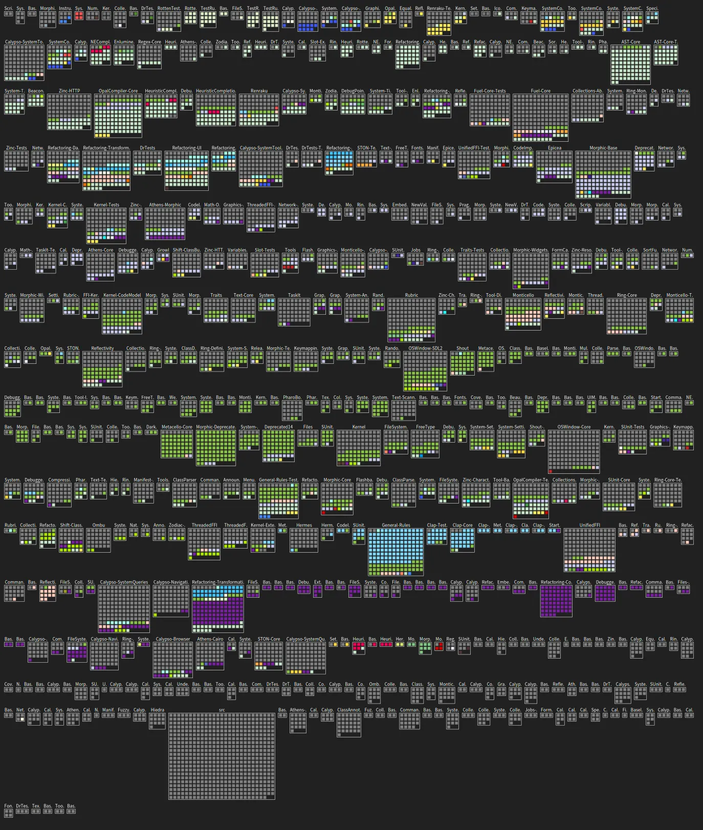
Again, the visualisation well presents the different packages and the one with major author.
The gray square corresponds to file less modified in the system the last two years.