In this post, we will be looking at how to use a Tree-Sitter grammar to help build a parser for a language.
We will use the Perl language example for this.
Note: Creating a parser for a language is a large endehavour that can easily take 3 to 6 months of work.
Tree-Sitter, or any other grammar tool, will help in that, but it remains a long task.
do make (note: it gave me some error, but the library file was generated all the same)
(on Linux) it creates a libtree-sitter-perl.so dynamic library file.
This must be moved in some standard library path (I chose /usr/lib/x86_64-linux-gnu/ because this is where the libtree-sitter.so file was).
Pharo uses FFI to link to the grammar library, that’s why it’s a good idea to put it in a standard directory.
You can also put this library file in the same directory as your Pharo image, or in the directory where the Pharo launcher puts the virtual machines.
The subclasses of FFILibraryFinder can tell you what are the standard directories on your installation.
For example on Linux, FFIUnix64LibraryFinder new paths returns a list of paths that includes '/usr/lib/x86_64-linux-gnu/' where we did put our grammar.so file.
We use the Pharo-Tree-Sitter project (https://github.com/Evref-BL/Pharo-Tree-Sitter) of Berger-Levrault, created by Benoit Verhaeghe, a regular contributor to Moose and this blog.
You can import this project in a Moose image following the README instructions.
Notice that we gave the name of the dynamic library file created above (libtree-sitter-perl.so).
If this file is in a standard library directory, FFI will find it.
We can now experiment “our” parser on a small example:
parser := TSParser new.
tsLanguage := TSLanguage perl.
parser language: tsLanguage.
string :='# this is a comment
my $var = 5;
'.
tree := parser parseString: string.
tree rootNode
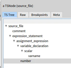
This gives you the following window:
That looks like a very good start!
But we are still a long way from home.
Let’s look at a node of the tree for fun.
node := tree rootNode firstNamedChild will give you the first node in the AST (the comment).
If we inspect it, we see that it is a TSNode
we can get its type: node type returns the string 'comment'
node nextSibling returns the next TSNode, the “expression-statement”
node startPoint and node endPoint tell you where in the source code this node is located.
It returns instances of TSPoint:
node startPoint row = 0 (0 indexed)
node startPoint column = 0
node endPoint row = 0
node endPoint column = 19
That is to say the node is on the first row, extending from column 0 to 19.
With this, one could get the text associated to the node from the original source code.
That’s it for today.
In a following post we will look at doing something with this AST using the Visitor design pattern.
When it comes to understand a software system, we are often focusing on the software artifact itself.
What are the classes? How they are connected with each other?
In addition to this analysis of the system, it can be interesting to explore how the system evolves through time.
To do so, we can exploit its git history.
In Moose, we developed the project GitProjectHealth that enables the analysis of git history for projects hosted by GitHub, GitLab, or BitBucket.
The project also comes with a set of metrics one could use directly.
For this first blog post, we will experiment GitProjectHealth on the Famix project.
Since this project is a GitHub project, we first create a GitHub token that will give GitProjectHealth the necessary authorization.
Then, we import the moosetechnology group (that hosts the Famix project).
group := githubImporter importGroup: 'moosetechnology'.
This first step allows us to get first information on projects.
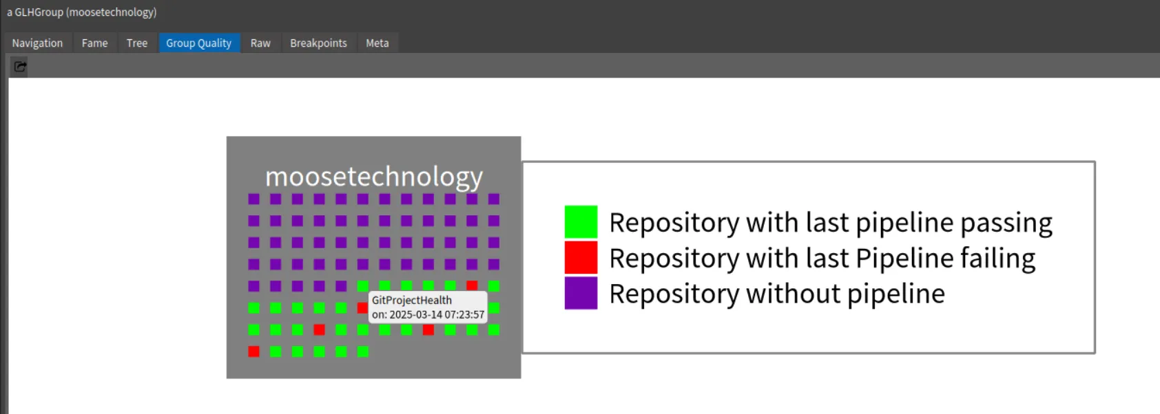
For instance, by inspecting the group, we can select the “Group quality” view and see the group projects and the last status of their pipelines.
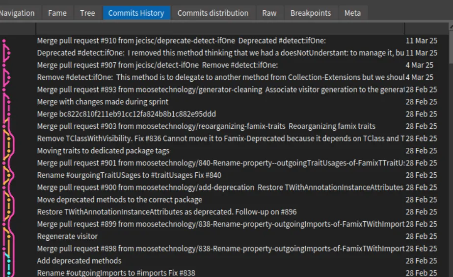
Then, by navigating to the Famix project and its repository, you can view the Commits History.
.
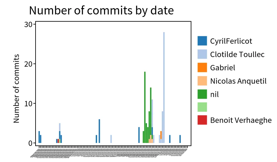
It is also possible to explore the recent commit distribution by date and author
.
In this visualization, we discover that the most recent contributors are “Clotilde Toullec” and “CyrilFerlicot”.
The “nil” refers to a commit authors that did not fill GitHub with their email. It is anquetil (probably the same person as “Nicolas Anquetil”).
The square without name is probably someone that did not fill correctly the local git config for username.
A popular metric when looking at git history is the code churn.
Code churn refer to edit of code introduced in the past.
It corresponds to the percentage of code introduced in a commit and then modified in other comments during a time period (e.g in the next week).
However many code churn definitions exit.
The first step is thus to discover what commits modified my code.
To do so, we implemented in GitProjectHealth information about diff in commit.
To extract this information, we first ask GitProjectHealth to extract more information for the commits of the famix project.
famix := group projects detect: [ :project| project name ='Famix' ].
"I want to go deeper in analysis for famix repository, so I complete commit import of this project"
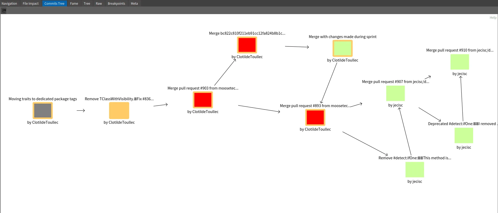
Then, when inspecting a commit, it is possible to switch to the “Commits tree” view.
Here how to read to above example
The orange square “Remove TClassWithVisibility…” is the inspected commit.
The gray square is the parent commit of the selected ones.
The red squares are subsequent commits that modify at least one file in common with the inspected commit
The green squares are commits that modifies other part of the code
Based on this example, we see that Clotilde Toullec modifies code introduced in selected commits in three next commits.
Two are Merged Pull Request.
This can represent linked work or at least actions on the same module of the application.
It is possible to go even deeper in the analysis by connecting GitProjectHealth with other analysis.
This is possible by connecting metamodels.
For instance, it is possible to link GitProjectHealth with Jira system, of Famix models.
You can look at the first general documentation, or stay tune for the next blog post about GitProjectHealth!
Control Flow Graphs (CFG) are a common tool for static analyzis of a computation unit (eg. a method) and find some errors (unreachable code, infinite loops)
It is based on the concept of Basic Block: a sequence of consecutive statements in which flow of control can only enter at the beginning and leave at the end. Only the last statement of a basic block can be a branch statement and only the first statement of a basic block can be a target of a branch.
There are two distinctive basic blocks:
Start Block: The entry block allows the control to enter into the control flow graph. There should be only one start block.
Final Block: Control flow leaves through the exit block. There may be several final blocks.
The package FAST-Fortran-Analyses in https://github.com/moosetechnology/FAST-Fortran contains classes to build a CFG of a Fortran program unit (a main program, a function, or a subroutine).
We must first create a FAST model of a Fortran program.
For this we need an external parser.
We currently use fortran-src-extras from https://github.com/camfort/fortran-src-extras.
This will produce a json AST of the program that we can turn into a FAST-Fortran AST.
If you have fortran-src-extras installed on your computer, all this is automated in FAST-Fortran
<fortran-file.f> asFileReference
readStreamDo: [ :st|
FortranProjectImporter new getFASTFor: st contents ]
This script will create an array of ASTs from the <fortran-file.f> given fortran file.
If there are several program units in the file, there will be several FAST models in this array.
In the example below, there is only one program, so the list contains only the AST for this program.
We will use the following Fortran-77 code:
PROGRAM EUCLID
* Find greatest common divisor using the Euclidean algorithm
This visitor goes throught the FAST model and creates a list of basic blocks that can be inspected with the #basicBlocks method.
There is a small hierarchy of basic block classes:
FASTFortranAbstractBasicBlock, the root of the hierarchy.
It contains #statements (which are FAST statement nodes).
It has methods to test its nature: isStart, isFinal, isConditional.
It defines an abstract method #nextBlocks that returns a list of basic blocks that this one can directly reach.
Typically there are 1 or 2 next blocks, but Fortran can have more due to “arithmetic IF”, “computed GOTO” and “assigned GOTO” statements.
FASTFortranBasicBlock, a common basic block with no branch statement.
If it is final, its #nextBlocks is empty, otherwise it’s a list of 1 block.
FASTFortranConditionalBasicBlock, a conditional basic block.
It may reach several #nextBlocks, each one associated with a value, for example true and false.
The method #nextBlockForValue: returns the next block associated to a given value.
In our version of CFG, a conditional block may only have one statement (a conditional statement).
You may have noticed that our blocks are a bit different from the definition given at the beginning of the blog-post:
our “common” blocs cannot have several next, they never end with a conditional statement;
our conditional blocks can have only one statement.
For the program above, the CFG has 10 blocks.
the first block is a common block and contains 2 statements, the PRINT and the READ;
its next bloc is a conditional block for the IF.
It has 2 next blocs:
true leads to a common block with 2 statements, the PRINT and the STOP. This is a final block (STOP ends the program);
As a first analysis tool, we can visualize the CFG.
Inspecting the result of the next script will open a Roassal visualization on the CFG contained in the FASTFortranCFGVisitor.
FASTFortranCFGVisualization on: <aFASTFortranCFGVisitor>
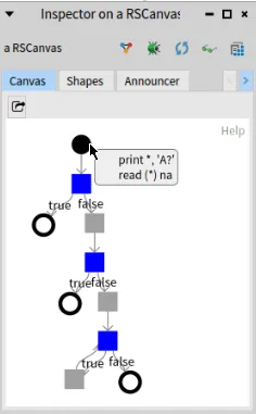
For the program above, this gives the visualization below.
the dark dot is the starting block (note that it is a block and contains statements);
the hollow dots are final blocks;
it’s not the case here, but a block may also be start and final (if there are no conditional blocks in the program) and this would be represented by a “target”, a circle with a dot inside;
a grey square is a comon block;
a blue square is a conditional block;
hovering the mouse on a block will bring a pop up with the list of its statements (this relies on the FASTFortranExporterVisitor)
One can see that:
the start block has 2 associated statements (PRINT and READ);
there are several final blocks, due to the STOP statements;
there is a loop at the bottom left of the graph where the last blue conditional block is “IF (IB.NE.0)” and the last statement of the grey block (true value of the IF), is a GOTO.
There are little analyses for now on the CFG, but FASTFortranCFGChecker will compute a list of unreachableBlocks that would represent dead code.
Control flow graphs may also be used to do more advanced analyses and possibly refactor code.
For example, we mentioned the loop at the end of our program implemented with a IF statement and a GOTO.
This could be refactored into a real WHILE loop that would be easier to read.
This is left as an exercise for the interested people 😉
Building a control flow graph is language dependant to identify the conditional statements, where they lead, and the final statements.
But much could be done in FAST core based on FASTTReturnStatement and a (not yet existing at the time of writing) FASTTConditionalStatement.
Inspiration could be taken from FASTFortranCFGVisitor and the process is not overly complicated.
It would probably be even easier for modern languages that do not have the various GOTO statements of Fortran.
Once the CFG is computed, the other tools (eg. the visualization) should be completely independant of the language.
These tools may be usable directly on a specific language FAST meta-model, or might require some adjustements by subtyping them.
They are not out-of-the-shelf ready to use stuff, but they can provide good inspiration for whatever you need to do.
Writing test for FAST can be pretty tedious because you have to build a FAST model in the test corresponding to your need.
It often has a lot of nodes that you need to create in the right order with the right properties.
This is where FASTDumpVisitor can help by visiting an existing AST and “dump” it as a string.
The goal is that executing this string in Pharo should recreate exactly the same AST.
Dumping an AST can also be useful to debug an AST and checking that it has the right properties.
To use it, you can just call FASTDumpVisitor visit: <yourAST> and print the result. For example:
FASTDumpVisitor visit:
(FASTJavaUnaryExpression new
operator: '-' ;
expression:
(FASTJavaIntegerLiteral new
primitiveValue: '5'))
will return the string:
FASTJavaUnaryExpression new expression:(FASTJavaIntegerLiteral new primitiveValue:'5');operator:'-' which, if evaluated, in Pharo will recreate the same AST as the original.
Note: Because FAST models are actually Famix models (Famix-AST), the tools works also for Famix models.
But Famix entities typically have more properties and the result is not so nice:
FASTDumpVisitor visit:
(FamixJavaMethod new
name: 'toto' ;
parameters: {
FamixJavaParameter new name: 'x' .
FamixJavaParameter new name: 'y'} ).
will return the string: FamixJavaMethod new parameters:{FamixJavaParameter new name:'x';isFinal:false;numberOfLinesOfCode:0;isStub:false.FamixJavaParameter new name:'y';isFinal:false;numberOfLinesOfCode:0;isStub:false};isStub:false;isClassSide:false;isFinal:false;numberOfLinesOfCode:-1;isSynchronized:false;numberOfConditionals:-1;isAbstract:false;cyclomaticComplexity:-1;name:'toto'.
By definition an AST (Abstract Syntax Tree) is a tree (!).
So the same variable can appear several time in an AST in different nodes (for example if the same variable is accessed several times).
The idea of the class FASTLocalResolverVisitor is to relate all uses of a symbol in the AST to the node where the symbol is defined.
This is mostly useful for parameters and local variables inside a method, because the local resover only looks at the AST itself and we do not build ASTs for entire systems.
This local resolver will look at identifier appearing in an AST and try to link them all together when they correspond to the same entity.
There is no complex computation in it.
It just looks at names defined or used in the AST.
This is dependant on the programming language because the nodes using or defining a variable are not the same in all languages.
For Java, there is FASTJavaLocalResolverVisitor, and for Fortran FASTFortranLocalResolverVisitor.
The tool brings an extra level of detail by managing scopes, so that if the same variable name is defined in different loops (for example), then each use of the name will be related to the correct definition.
The resolution process creates:
In declaration nodes (eg. FASTJavaVariableDeclarator or FASTJavaParameter),a property #localUses will list all referencing nodes for this variable;
In accessing nodes, (eg. FASTJavaVariableExpression), a property #localDeclarations will lists the declaration node corresponding this variable.
If the declaration node was not found a FASTNonLocalDeclaration is used as the declaration node.
Note: That this looks a bit like what Carrefour does (see /blog/2022-06-30-carrefour), because both will bind several FAST nodes to the same entity.
But the process is very different:
Carrefour will bind a FAST node to a corresponding Famix node;
The local resolver binds FAST nodes together.
So Carrefour is not local, it look in the entire Famix model to find the entity that matches a FAST node.
In Famix, there is only one Famix entity for one software entity and it “knows” all its uses (a FamixVariable has a list of FamixAccess-es).
Each FAST declaration node will be related to the Famix entity (the FamixVariable) and the FAST use nodes will be related to the FamixAccess-es.
On the other hand, the local resolver is a much lighter tool.
It only needs a FAST model to work on and will only bind FAST nodes between themselves in that FAST model.
For round-trip re-engineering, we need to import a program in a model, modify the model, and re-export it as a (modified) program.
A lot can go wrong or be fogotten in all these steps and they are not trivial to validate.
First, unless much extra information is added to the AST, the re-export will not be syntactically equivalent: there are formatting issues, indentation, white spaces, blank lines, comments that could make the re-exported program very different (apparently) from the original one.
The class FASTDifferentialValidator helps checking that the round-trip implementation works well.
It focuses on the meaning of the program independently of the formatting issues.
The process is the follwing:
parse a set of (representative) programs
model them in FAST
re-export the programs
re-import the new programs, and
re-create a new model
Hopefully, the two models (2nd and last steps) should be equivalent
This is what this tool checks.
Obviously the validation can easily be circumvented.
Trivially, if we create an empty model the 1st time, re-export anything, and create an empty model the second time, then the 2 models are equivalent, yet we did not accomplish anything.
This tool is an help for developers to pinpoint small mistakes in the process.
Note that even in the best of conditions, there can still be subtle differences between two equivalent ASTs.
For example the AST for “a + b + c” will often differ from that of “a + (b + c)”.
The validator is intended to run on a set of source files and check that they are all parsed and re-exported correctly.
It will report differences and will allow to fine tune the comparison or ignore some differences.
It goes through all the files in a directory and uses an importer, an exporter, and a comparator.
The importer generates a FAST model from some source code (eg. JavaSmaCCProgramNodeImporterVisitor); the exporter generates source code from a model (eg. FASTJavaExportVisitor); the comparator is a companion class to the DifferentialValidator that handle the differences between the ASTs.
The basic implementation (FamixModelComparator) does a strict comparison (no differences allowed), but it has methods for accepting some differences:
#ast: node1 acceptableDifferenceTo: node2:
If for some reason the difference in the nodes is acceptable, this method must return true and the comparison will restart from the parent of the two nodes as if they were the same.
#ast: node1 acceptableDifferenceTo: node2 property: aSymbol.
This is for property comparison (eg. the name of an entity), it should return nil if the difference in value is not acceptable and a recovery block if it is acceptable. Instead of resuming from the parent of the nodes, the comparison will resume from an ancestor for which the recovery block evaluates to true.
Tags can be a powerful tool to visualize things on legacy software and perform analyses.
For example, tags can be used to create virtual entities and see how they “interact” with the real entities of the system analyzed.
In the article Decomposing God Classes at Siemens we show how tags can be used to create virtual classes and see their dependencies to real classes.
In this post I will show another use of tags: how they can materialize a concept and show its instantiation in a system.
The scenario is that of analysing Corese, a platform to “create, manipulate, parse, serialize, query, reason and validate RDF data.”
Corese is an old software that dates back to the early days of Java.
Back then, enums did not exist in Java and a good way to implement them was to use a set of constants:
publicstaticfinalintMONDAY=1;
publicstaticfinalintTUESDAY=2;
publicstaticfinalintWEDNESDAY=3;
publicstaticfinalintTHURSDAY=4;
publicstaticfinalintFRIDAY=5;
publicstaticfinalintSATURDAY=6;
publicstaticfinalintSUNDAY=7;
Those were the days!
As an effort to restructure and rationalize implementation, the developers of Corese wish to replace these sets of constants by real Java enums.
This is not something that can be done in any modern IDE even with the latest refactoring tool.
For an analysis in Moose, we need a model of the system, and this starts with getting the source code (https://github.com/corese-stack/corese-core).
The model is created using VerveineJ which can be run using docker:
docker run -rm -v src/main/java/:/src ghcr.io/evref-bl/verveinej:latest -alllocals -o corese-core.json
This will create a file corese-core.json in the directory src/main/java/.
The command to create the model as an option -alllocals.
This is because VerveineJ by default only tracks the uses of variables with non primitive type (variables containing objects).
Here the constants are integers and if we want to know where they are used, we need more details.
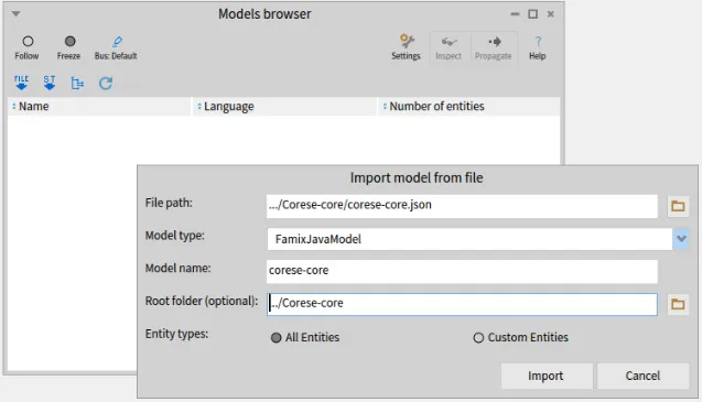
Let’s import the model in Moose.
This can be done simply by dragging-and-dropping the file in Moose.
We will study the use of the constants defined in fr.inria.corese.core.stats.IStats:
publicinterfaceIStats {
publicstaticfinalintNA=0;
publicstaticfinalintSUBJECT=1;
publicstaticfinalintPREDICATE=2;
publicstaticfinalintOBJECT=3;
publicstaticfinalintTRIPLE=4;
[...]
To find where the constants are used, we need to find the representation of the constants in the model.
For this, we can inspect the model (“Inspect” button in the Model Browser) and look for all “Model Attributes”.
The constants are attributes of the interface/class in which they are defined as shown in the listing above).
And they are model attributes because they are defined in the source code analysed, as opposed to System.out which may be used in the code but for which we don’t have the source code.
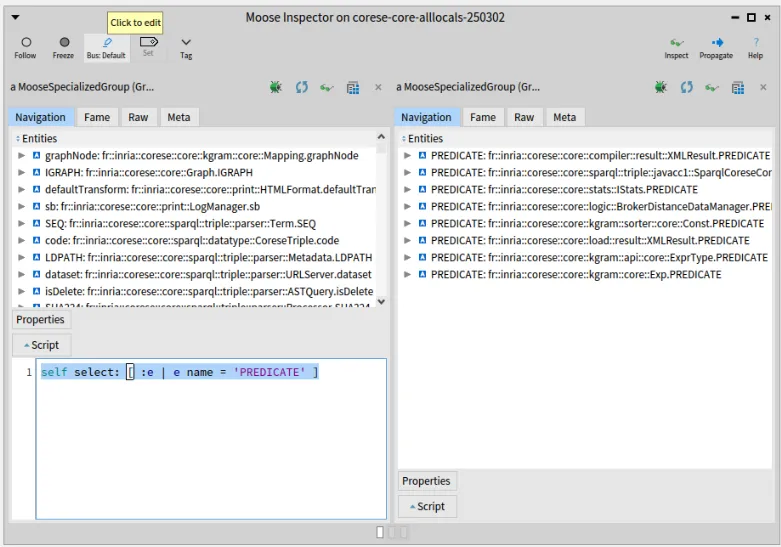
We can then select all the model attributes named PREDICATE:
select: [ :each | each name = 'PREDICATE'].
(note, the backslash (\) before the square bracket ([) was added by the publishing tool and is not part of the code)
Moose gives us 8 different definitions of PREDICATE (and 9 for OBJECT, and 10 for SUBJECT).
The one we are interested in is the 3rd in the list (IStats.PREDICATE).
Having the same constants defined multiple times is not good news for the analysis and for the developers.
But this kind of thing is fairly common in old systems which evolved during a long time in the hands of many developers.
Not all of them had a complete understanding of the system and each had different skills and programming habits.
Looking at the lists of definitions for the 3 main constants (SUBJECT, PREDICATE, OBJECT), we find that there are at least 5 different definitions of these constants:
stats.IStats:
publicstaticfinalintNA=0;
publicstaticfinalintSUBJECT=1;
publicstaticfinalintPREDICATE=2;
publicstaticfinalintOBJECT=3;
publicstaticfinalintTRIPLE=4;
kgram.sorter.core.Const:
publicstaticfinalintALL=0;
publicstaticfinalintSUBJECT=1;
publicstaticfinalintPREDICATE=2;
publicstaticfinalintOBJECT=3;
publicstaticfinalintTRIPLE=4;
publicstaticfinalintNA=-1;
compiler.result.XMLResult
privatestaticfinalintTRIPLE=9;
privatestaticfinalintSUBJECT=10;
privatestaticfinalintPREDICATE=11;
privatestaticfinalintOBJECT=12;
kgram.api.core.ExprType
publicstaticintTRIPLE=88;
publicstaticintSUBJECT=89;
publicstaticintPREDICATE=90;
publicstaticintOBJECT=91;
kgram.core.Exp
publicstaticfinalintANY=-1;
publicstaticfinalintSUBJECT=0;
publicstaticfinalintOBJECT=1;
publicstaticfinalintPREDICATE=2;
So now we need to track the uses of all these constants in the system to understand how they can be replaced by one enum.
Note: Don’t close the Inspector window yet, we are going to need it soon.
Moose can help us here with tags.
Tags are (as the name implies) just labels that can be attached to any entity in the model.
Additionally, tags have a color that will help us distinguish them in visualizations.
So let’s tag our constants.
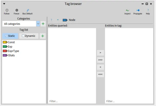
We will define 5 tags, one for each set of constants, that is to say one for each of the 5 classes that implement these constants.
You can choose whatever name and color you prefer for your tags, as long as you remember which is which.
Here I named the tags from the name of the classes that define each set of constant.
Now we want to tag all the constants in a set with the same tag.
Let’s see how to do it for constants in IStats, the ones listed in the previous section and that were our initial focus.
We select the “IStats” tag in the Tag Browser and go back to the Inspector where we have a list of all definitions of PREDICATE.
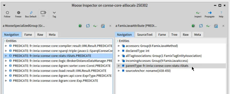
If we click on the 3rd of these PREDICATE (“fr::inria::corese::core::stats::IStats.PREDICATE”), a new pane appears on the right, focusing on this attribute.
There, we can click on its “parentType”, giving yet another pane.
(The following screenshot shows the inspector right before we click on “parentType”).
.
The right pane now focuses on the IStats Java interface.
We can click on “attributes” to get the list of attributes it defines (including PREDICATE from which we started).
There are 5 attributes which are the ones listed in the previous section.
So far so good.
To tag these attributes, we will “propagate” them (toolbar button of the Inspector on the right) to all tools that are in “Follow” mode.
Note that if you minimized the Tag Browser at some point, it will be in “Freeze” mode like in the screenshot above.
You need to put it back in “Follow” (radio toolbar button on the left) before propagating the list of constants.
Once propagated, the list appears in the center pane of the Tag Browser and you can pass it to the right pane with the ”>>>” button.
Doing this will effectively tag the entities with the selected tag.
We now have tagged these 5 constants with the “IStats” tag.
Ideally we want to find also the usage of these constants.
So we would like to also tag the methods that use these constants.
For this you can open a Query Browser, it will start with the same list of 5 attributes that we just propagated.
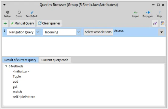
We can create a “Navigation query” and ask for all the “incoming” “accesses” to these attributes as shown below.
The result is a list of 6 methods.
We can now propagate these 6 methods and they will appear in the Tag Browser.
We tag them with the same tag as the attributes themselves.
You can repeat the same operations for the 5 sets of constants listed above and the 5 different tags.
All this tagging was to be able to visualize where each set of constant is defined and, most importantly, used.
We now turn to the “Architectural Map” which is a fine tool to visualize tags.
for example, we could show all the top level packages of Corese and the Architectural Map will give visual clues on which ones contain tagged entities, and what tags.
The Architectural Map allows to expand the content of entities which will allow us to deep dive into each package containing tagged entities to understand where exactly the entities is used or defined.
To select all the top level packages, we go back one last time to the Inspector to the very first pane on the left (you may also “Inspect” again the model to open a new Inspector).
We select the “Model packages” and enter this query in the “script” at the bottom: self select: [ :each | each parentPackage isNotNil and: [each parentPackage name = 'core'] ].
(Again, ignore the backslashes)
The result is a list of 23 packages that we can propagate.
Finally we open an Architectural Map that will start with the 23 packages that we just propagated.
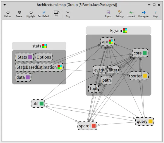
In the following screenchot, I restricted the Architectural Map to the only 5 packages that do use our tags: “stats”, “kgram”, “util”, “sparql”, and “query”.
This makes it easier to see the results here.
I also expanded “kgram” that is small and contains different tags.
The single-color square, on the right of each package name, shows that it contains entities having one uniq tag (of this color).
In our case it means that it contains the constants and methods accessing them, all with the same tag.
For example, “core” and “util” packages contain entities tagged with only the green tag (which corresponds to the kgram.core.Exp class as previously shown in the Tag Browser screenshot).
When the square is multicolored, it means it contains entities with different tags.
For example, we see that the package “kgram” contains at least the green (“Exp”) and the yellow (“Const”) tags.
Note that in this particular case, I added another tag for class kgram.api.core.Node which has its own definition of the OBJECT constant.
I wanted to see where it was used also.
This is the reason for the multicolored square of class StatsBasedEstimation, in package “stats”, which uses OBJECT from Node and the other constants from IStats.
In the end, the visualization allows to conclude that each package sticks pretty much to its own definition of the constants which is rather reassuring.
It also shows where one would have to look if we were to replace the constant by a real enum.
This is not the end of it however because the constant values used in these methods can be passed off to other methods as argument.
Here Famix alone (the meta-model used in Moose by default) can no longer help us to follow the flow of usage of the constants because they are just integer being passed around.
For a finer analysis, a complete AST model should be used.
This could be done with the FAST meta-model (Famix-AST), but it is another story that falls outside the scope of this blog-post.



 .
. .
.
 .
.