Some tools on FAST models
The package FAST-Core-Tools in repository https://github.com/moosetechnology/FAST offers some tools or algorithms that are running on FAST models.
These tools may be usable directly on a specific language FAST meta-model, or might require some adjustements by subtyping them. They are not out-of-the-shelf ready to use stuff, but they can provide good inspiration for whatever you need to do.
Dumping AST
Section titled “Dumping AST”Writing test for FAST can be pretty tedious because you have to build a FAST model in the test corresponding to your need. It often has a lot of nodes that you need to create in the right order with the right properties.
This is where FASTDumpVisitor can help by visiting an existing AST and “dump” it as a string.
The goal is that executing this string in Pharo should recreate exactly the same AST.
Dumping an AST can also be useful to debug an AST and checking that it has the right properties.
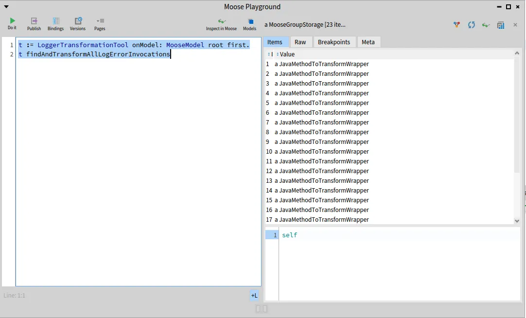
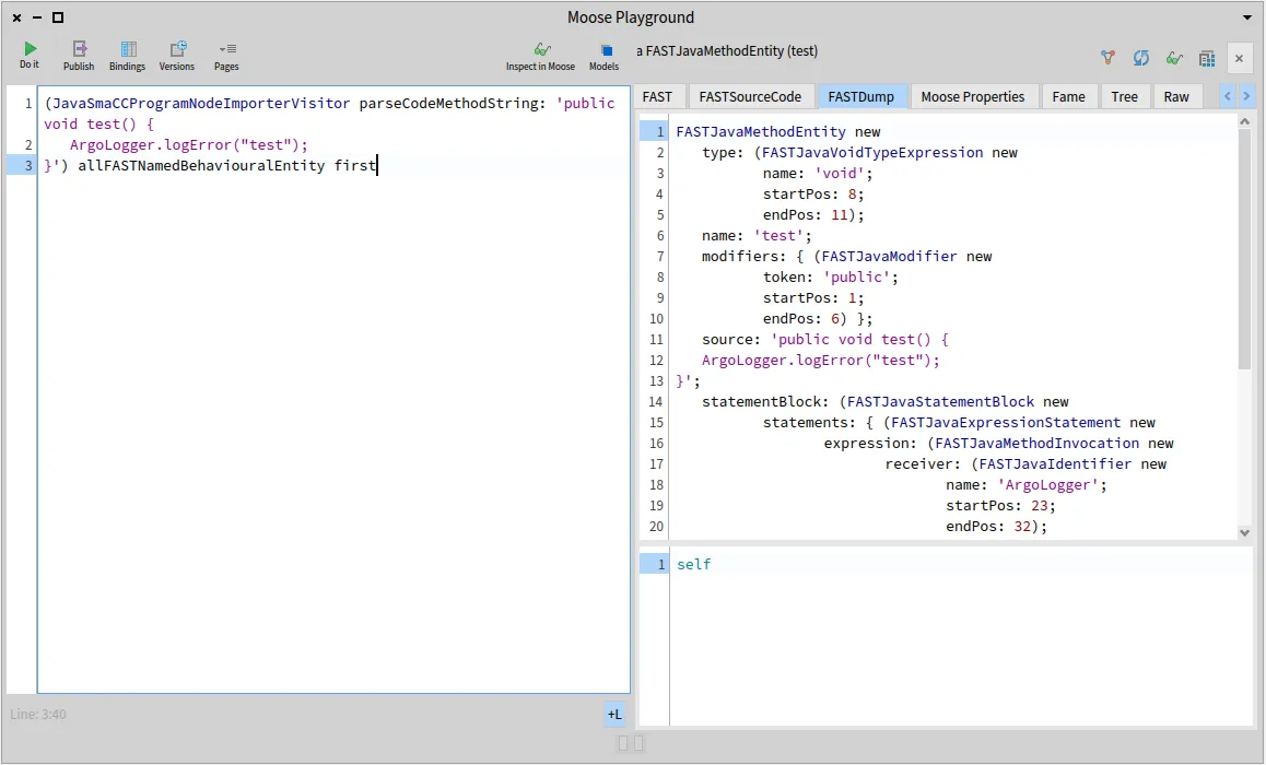
To use it, you can just call FASTDumpVisitor visit: <yourAST> and print the result. For example:
FASTDumpVisitor visit: (FASTJavaUnaryExpression new operator: '-' ; expression: (FASTJavaIntegerLiteral new primitiveValue: '5'))will return the string:
FASTJavaUnaryExpression new expression:(FASTJavaIntegerLiteral new primitiveValue:'5');operator:'-' which, if evaluated, in Pharo will recreate the same AST as the original.
Note: Because FAST models are actually Famix models (Famix-AST), the tools works also for Famix models. But Famix entities typically have more properties and the result is not so nice:
FASTDumpVisitor visit: (FamixJavaMethod new name: 'toto' ; parameters: { FamixJavaParameter new name: 'x' . FamixJavaParameter new name: 'y'} ).will return the string: FamixJavaMethod new parameters:{FamixJavaParameter new name:'x';isFinal:false;numberOfLinesOfCode:0;isStub:false.FamixJavaParameter new name:'y';isFinal:false;numberOfLinesOfCode:0;isStub:false};isStub:false;isClassSide:false;isFinal:false;numberOfLinesOfCode:-1;isSynchronized:false;numberOfConditionals:-1;isAbstract:false;cyclomaticComplexity:-1;name:'toto'.
Local symbol resolution in an AST
Section titled “Local symbol resolution in an AST”By definition an AST (Abstract Syntax Tree) is a tree (!). So the same variable can appear several time in an AST in different nodes (for example if the same variable is accessed several times).
The idea of the class FASTLocalResolverVisitor is to relate all uses of a symbol in the AST to the node where the symbol is defined.
This is mostly useful for parameters and local variables inside a method, because the local resover only looks at the AST itself and we do not build ASTs for entire systems.
This local resolver will look at identifier appearing in an AST and try to link them all together when they correspond to the same entity. There is no complex computation in it. It just looks at names defined or used in the AST.
This is dependant on the programming language because the nodes using or defining a variable are not the same in all languages.
For Java, there is FASTJavaLocalResolverVisitor, and for Fortran FASTFortranLocalResolverVisitor.
The tool brings an extra level of detail by managing scopes, so that if the same variable name is defined in different loops (for example), then each use of the name will be related to the correct definition.
The resolution process creates:
- In declaration nodes (eg.
FASTJavaVariableDeclaratororFASTJavaParameter),a property#localUseswill list all referencing nodes for this variable; - In accessing nodes, (eg.
FASTJavaVariableExpression), a property#localDeclarationswill lists the declaration node corresponding this variable. - If the declaration node was not found a
FASTNonLocalDeclarationis used as the declaration node.
Note: That this looks a bit like what Carrefour does (see /blog/2022-06-30-carrefour), because both will bind several FAST nodes to the same entity. But the process is very different:
- Carrefour will bind a FAST node to a corresponding Famix node;
- The local resolver binds FAST nodes together.
So Carrefour is not local, it look in the entire Famix model to find the entity that matches a FAST node. In Famix, there is only one Famix entity for one software entity and it “knows” all its uses (a FamixVariable has a list of FamixAccess-es). Each FAST declaration node will be related to the Famix entity (the FamixVariable) and the FAST use nodes will be related to the FamixAccess-es.
On the other hand, the local resolver is a much lighter tool. It only needs a FAST model to work on and will only bind FAST nodes between themselves in that FAST model.
Round-trip validation
Section titled “Round-trip validation”For round-trip re-engineering, we need to import a program in a model, modify the model, and re-export it as a (modified) program. A lot can go wrong or be fogotten in all these steps and they are not trivial to validate.
First, unless much extra information is added to the AST, the re-export will not be syntactically equivalent: there are formatting issues, indentation, white spaces, blank lines, comments that could make the re-exported program very different (apparently) from the original one.
The class FASTDifferentialValidator helps checking that the round-trip implementation works well.
It focuses on the meaning of the program independently of the formatting issues.
The process is the follwing:
- parse a set of (representative) programs
- model them in FAST
- re-export the programs
- re-import the new programs, and
- re-create a new model
Hopefully, the two models (2nd and last steps) should be equivalent This is what this tool checks.
Obviously the validation can easily be circumvented. Trivially, if we create an empty model the 1st time, re-export anything, and create an empty model the second time, then the 2 models are equivalent, yet we did not accomplish anything. This tool is an help for developers to pinpoint small mistakes in the process.
Note that even in the best of conditions, there can still be subtle differences between two equivalent ASTs. For example the AST for “a + b + c” will often differ from that of “a + (b + c)”.
The validator is intended to run on a set of source files and check that they are all parsed and re-exported correctly. It will report differences and will allow to fine tune the comparison or ignore some differences.
It goes through all the files in a directory and uses an importer, an exporter, and a comparator.
The importer generates a FAST model from some source code (eg. JavaSmaCCProgramNodeImporterVisitor); the exporter generates source code from a model (eg. FASTJavaExportVisitor); the comparator is a companion class to the DifferentialValidator that handle the differences between the ASTs.
The basic implementation (FamixModelComparator) does a strict comparison (no differences allowed), but it has methods for accepting some differences:
#ast: node1 acceptableDifferenceTo: node2: If for some reason the difference in the nodes is acceptable, this method must returntrueand the comparison will restart from the parent of the two nodes as if they were the same.#ast: node1 acceptableDifferenceTo: node2 property: aSymbol. This is for property comparison (eg. the name of an entity), it should returnnilif the difference in value is not acceptable and a recovery block if it is acceptable. Instead of resuming from the parent of the nodes, the comparison will resume from an ancestor for which the recovery block evaluates totrue.
 .
.